class: center, middle, inverse, title-slide .title[ # STA 235H - RCTs and Observational Studies ] .subtitle[ ## Fall 2023 ] .author[ ### McCombs School of Business, UT Austin ] --- <!-- <script type="text/javascript"> --> <!-- MathJax.Hub.Config({ --> <!-- "HTML-CSS": { --> <!-- preferredFont: null, --> <!-- webFont: "Neo-Euler" --> <!-- } --> <!-- }); --> <!-- </script> --> <style type="text/css"> .small .remark-code { /*Change made here*/ font-size: 80% !important; } .tiny .remark-code { /*Change made here*/ font-size: 90% !important; } </style> # Housekeeping - **.darkorange[Let's talk about ChatGPT]**. - Should be use as a *complement* of learning, not a *substitute*. - ChatGPT is mainly useful when you are able to check the *accuracy* of its answers. - You need to do your <u>own work</u>. -- - **.darkorange[No Office Hours this Thursday]**. - I will hold OH (for this week) on Tues (4pm - 5:30pm) and Wed (10:30am - 11:30am) --- # Last week .pull-left[ .center[ ] ] .pull-right[ - We talked about the **.darkorange[Ignorability Assumption]** - Started discussing **.darkorange[randomized controlled trials]**. - Why they are the gold standard. - How to analyze them. ] --- # Today .pull-left[ - Discuss about **.darkorange[limitations of RCTs]**: - Generalizability - Spillover/General equilibrium effects. - What is **.darkorange[selection on observables?]**: - Omitted Variable Bias - Regression Adjustment - Matching ] .pull-right[  ] --- background-position: 50% 50% class: left, bottom, inverse .big[ Limitations of RCTs ] --- # Recap - RCTs make the **.darkorange[ignorability assumption hold by design]** -- .box-4trans[How?] -- .center[ ] --- # Examples of RCTs .pull-left[ .center[  ] ] -- .pull-right[ .center[  ] ] --- # Steps to analyze a RCT? -- .pull-left-div3[ .box-4Trans[1) Check for balance] .box-4trans[(Remember to transform categorical variables into binary ones!)] ] -- .pull-center-div3[ .box-6Trans[2) Estimate diff.<br>in means] .box-6trans[(Simple regression<br>between `Y` and `Z`)] ] -- .pull-right-div3[ .box-7Trans[2)* Estimate diff. in means with covariates] .box-7trans[(Multiple regression between `Y` and `Z`, adding other baseline covariates `X`)] ] --- # Potential issues to have in mind -- .box-3trans[Generalizability of our estimated effects (External Validity)] -- - Where did we get our sample for our study from? Is it representative of a larger population? -- .box-5trans[Spillover effects] -- - Can an individual in the control group be affected by the treatment? -- .box-7trans[General equilibrium effects] -- - What happens if we scale up an intervention? Will the effect be the same? --- # External vs Internal Validity .center[ ] -- - Many times, RCTs use **.darkorange[convenience samples]** --- # SUTVA: No interference - Aside from **.darkorange[ignorability]**, RCTs rely on the **.darkorange[Stable Unit Treatment Value Assumption (SUTVA)]** -- .box-4Trans["The treatment applied to one unit does not affect the outcome for other units"] -- - No **.darkorange[spillovers]** - No **.darkorange[general equilibrium effects]** --- # Network effects (spillover) example - RCT where students where **.darkorange[randomized]** into two groups: - Treatment: Parents receive a text message when student misses school. - Control: Parents receive a general text message. -- - Estimate the **.darkorange[effect of the intervention on attendance]**. - Difference in average attendance between treated students and control students. -- - **.darkorange[Potential problem]**: Students usually skip school with a friend. -- .box-7trans[Why could this be a problem for causal inference?] --- # Network effects <br> .box-6LA[Can we do something about this?] <br> <br> -- 1. **.darkorange[Randomize at a higher level]** (e.g. neighborhood, school, etc. instead of at the individual level) -- 2. **.darkorange[Model the network!]** --- # General Equilibrium Effects - Usually arise when you **.darkorange[scale up]** a program or intervention. - Imagine you want to test the effect of providing information about employment and expected income to students to see whether it affect their choice of university and/or major. -- <br> <br> .box-7Trans[What could happen if you offer it to everyone?] --- background-position: 50% 50% class: middle, center .box-5Trans[Let's see another example] --- # Get Out The Vote .pull-left[ - "Get out the Vote" Large-Scale Mobilization experiment (Arceneaux, Gerber, and Green, 2006) - "Households containing one or two registered voters where **.darkorange[randomly assigned]** to treatment or control groups" - Treatment: GOTV phone calls - Stratified RCT: Two states divided into competitive and noncompetitive (randomized within state-competitiveness) ] .pull-right[  ] --- # Checking for balance .center[  ] --- <br> <br> <br> <br> <br> <br> .box-4LA[Let's go to R] --- # Estimating the effect - One important thing to note in the previous analysis is that **.darkorange[assignment to treatment]** `\(\neq\)` **.darkorange[contact]** ```r d_s1 %>% count(treat_real, contact) ``` ``` ## treat_real contact n ## 1 0 0 17186 ## 2 1 0 1626 ## 3 1 1 1374 ``` -- .box-5[Does this break the ignorability assumption?] -- - **.darkorange[Non-compliance]**: When the treatment assignment (e.g. calling the household) is not the same as the treatment (e.g. actually receiving a call/ making contact with the household) - What was **.darkorange[randomly assigned]** was calling the household. - Usually, <u>the effect of calling should be lower than the effect of actually receiving the call</u>. --- <br> <br> <br> <br> <br> .box-4[Can we do something if we can't randomize??] --- background-position: 50% 50% class: left, bottom, inverse .big[ Controlling by Confounders ] --- # Controlling by Confounders - We can control by a confounder by **.darkorange[including it in our regression]**: - After we control for it, we are doing a fair comparison (e.g. *"holding X constant"*) .box-4trans[Conditional Independence Assumption (CIA)] -- - *"<u>Conditional on X</u>, the ignorability assumption holds."* -- - But is there another way to control for confounders? -- .box-6Trans[Matching] --- # Matching Start with two groups: A treatment and a control group .center[ ] --- # Matching For each unit in the treatment group, let's find a similar unit in the control group .center[ 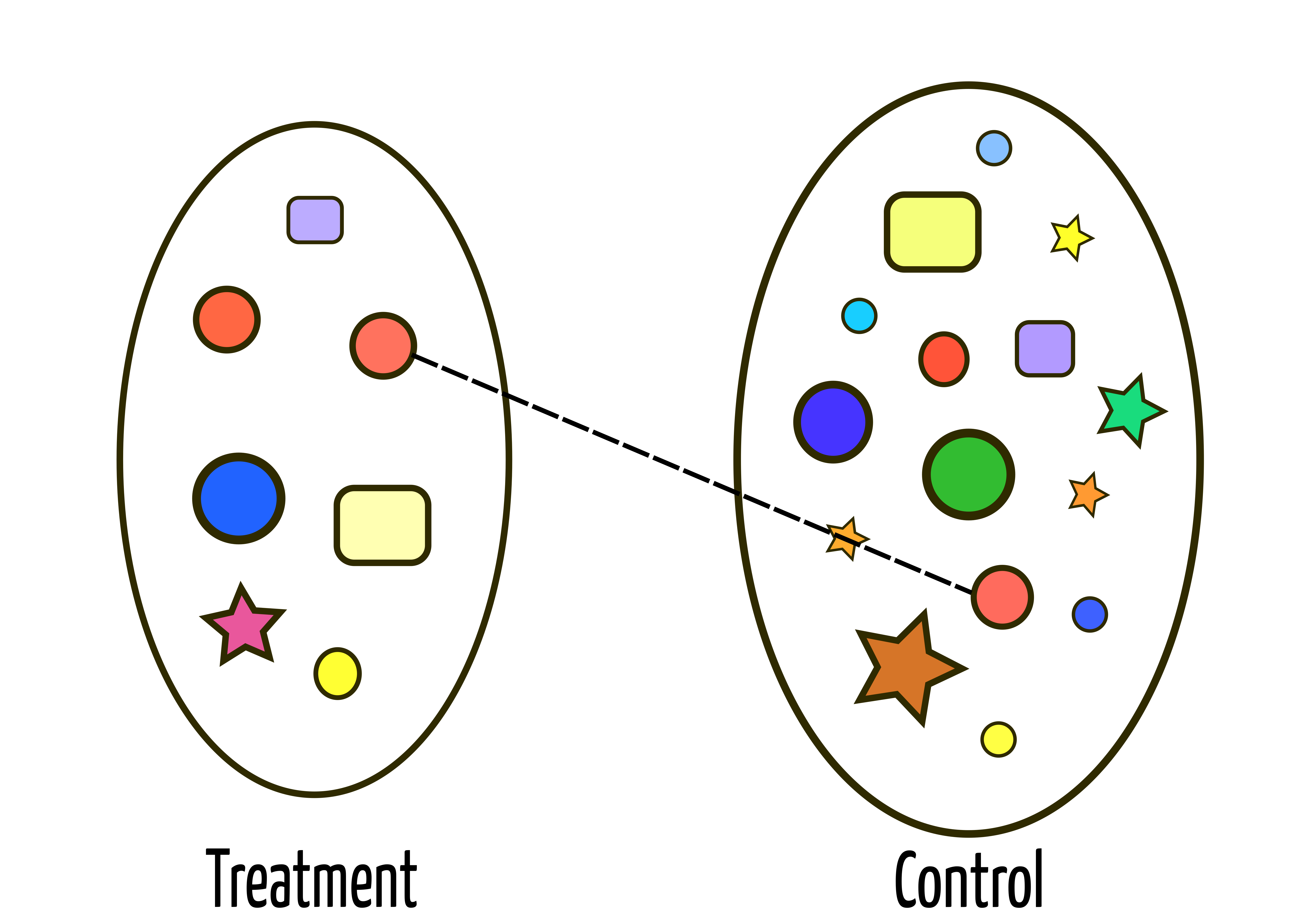] --- # Matching And we do this for all units .center[ 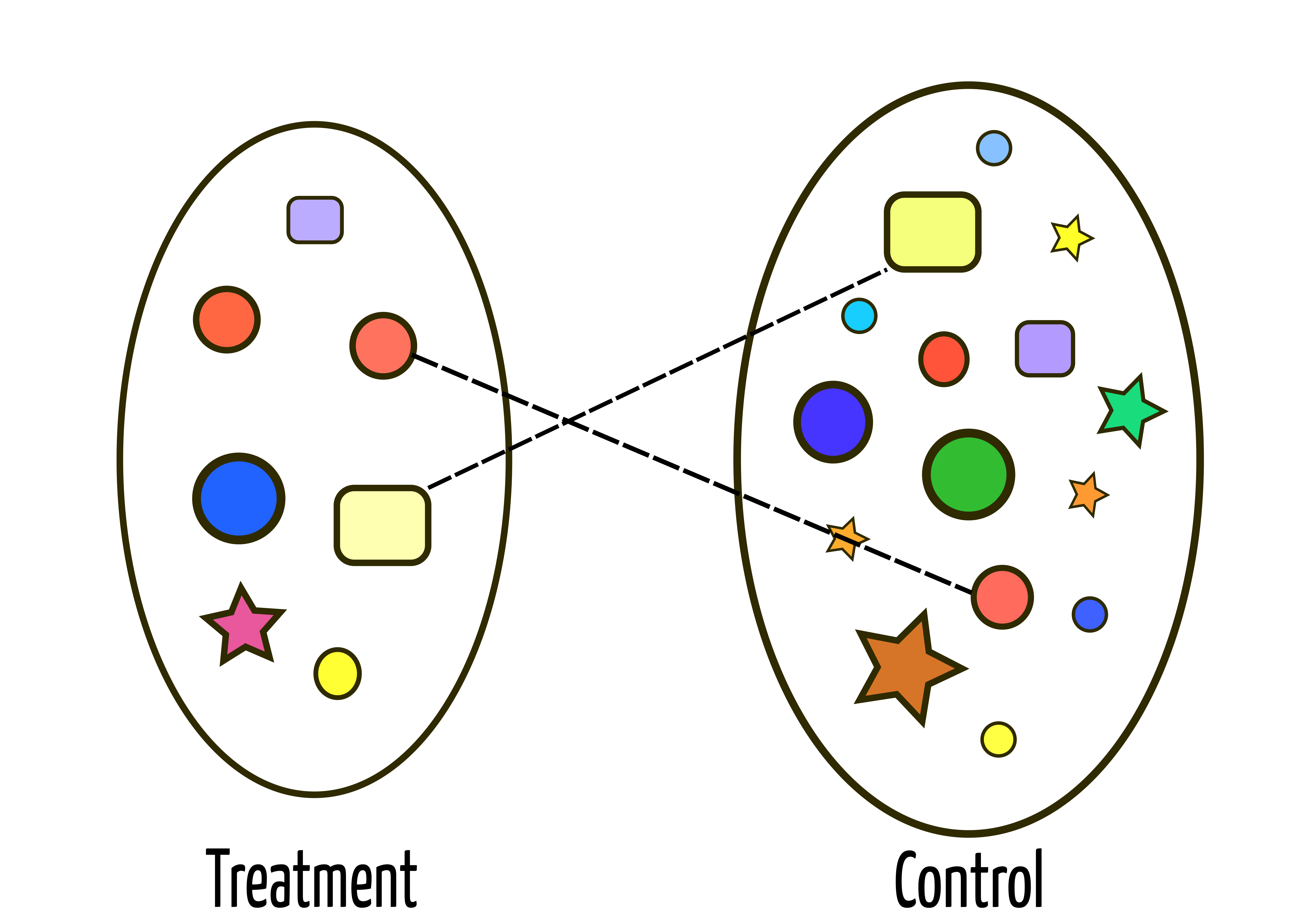] --- # Matching Note that we might not be able to find similar units for everyone! .center[ 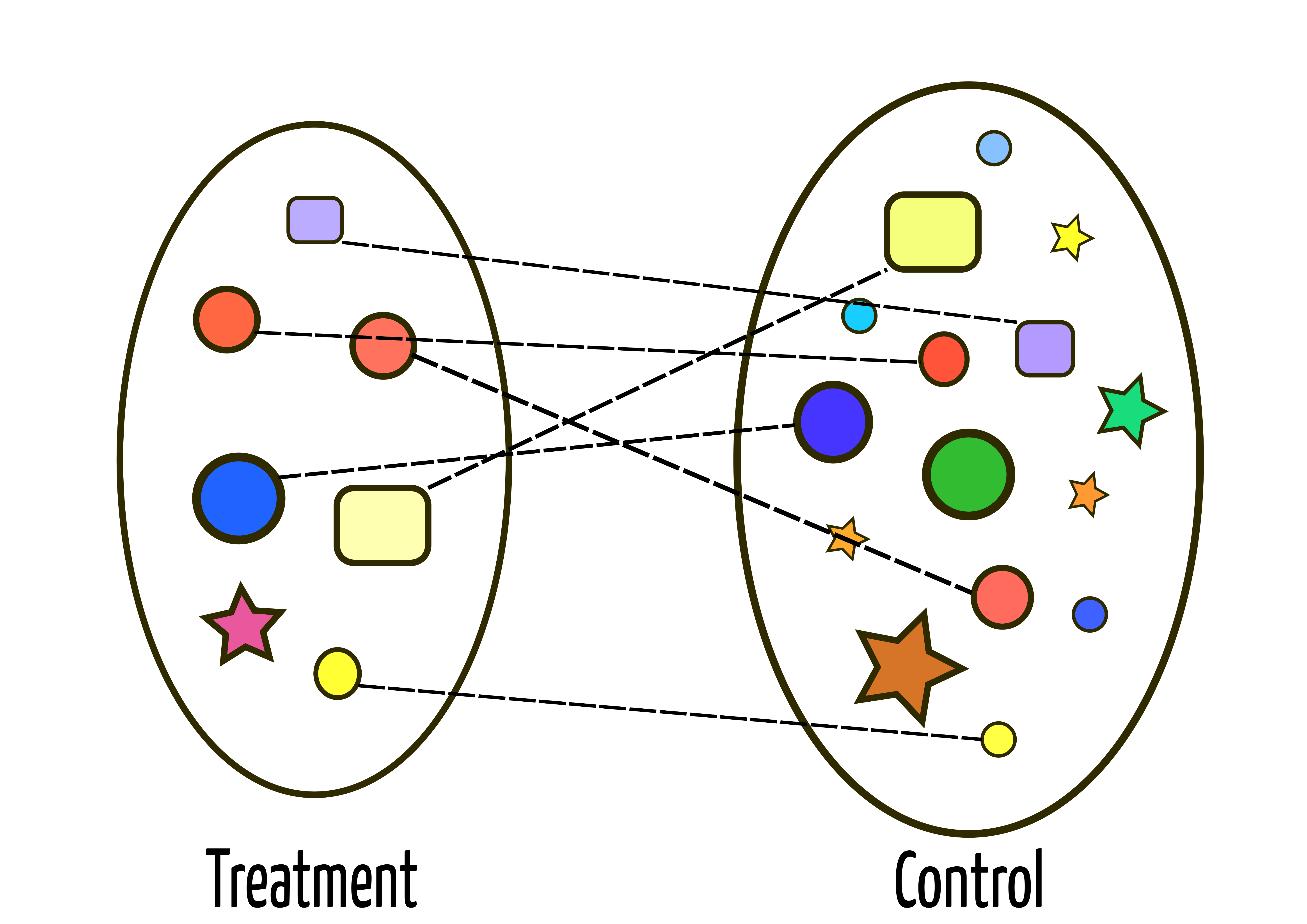] --- # Matching Then we just compare our matched groups .center[ 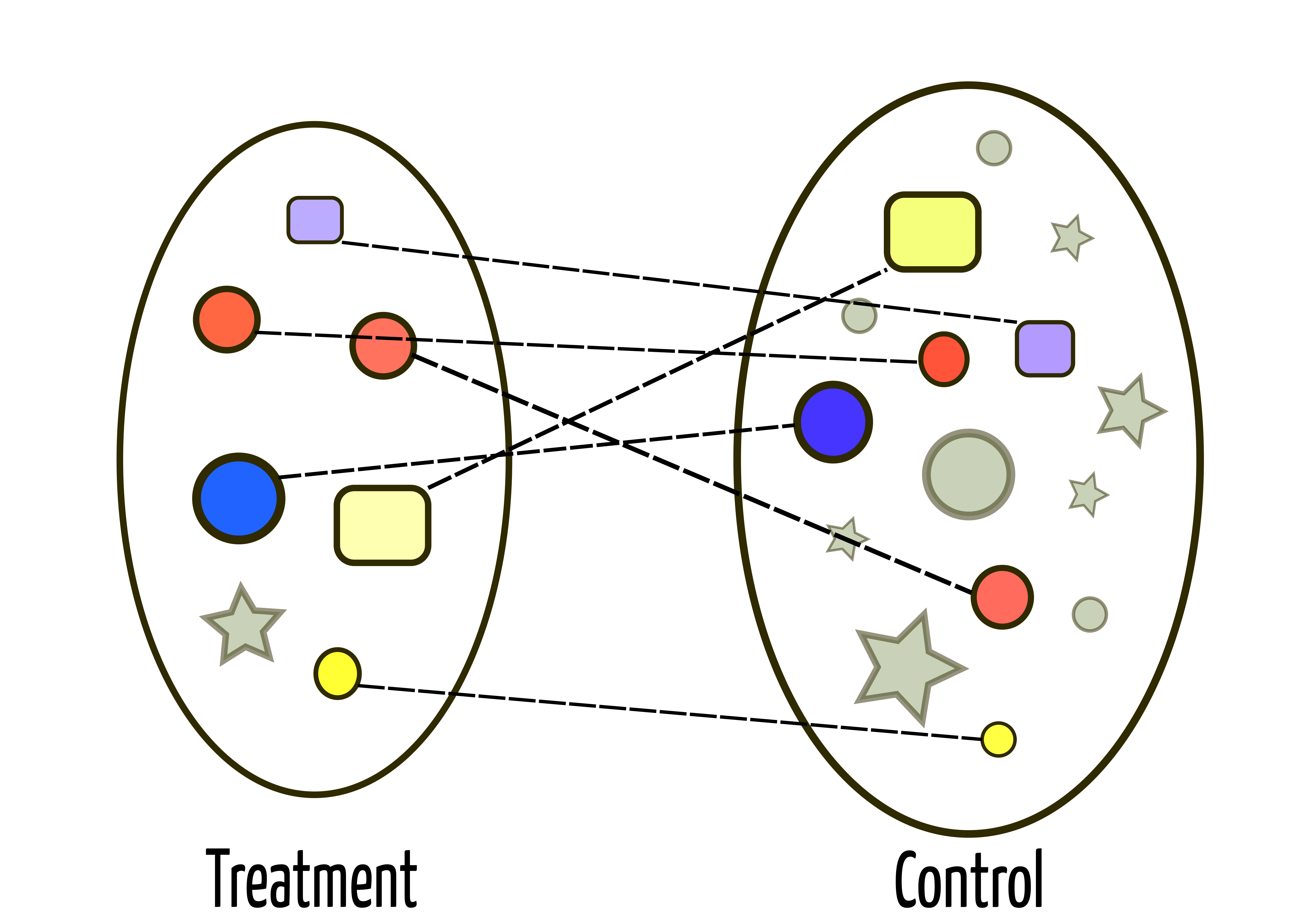] --- # Propensity Score Matching - It is **.darkorange[difficult (impossible) to match on all the variables we want]** (potential confounders) - The curse of dimensionality -- - **.darkorange[Propensity score]**: Probability of being in the treatment group given the individuals characteristics. `$$p = Pr(Z = 1) = \hat{\beta}_0 + \hat{\beta}_1X_1 + \hat{\beta}_2X_2 + ... + \hat{\beta}_kX_k$$` - E.g. Two units have a 50% chance of being treated, but one was <u>actually treated (Z=1)</u> and <u>the other one was not (Z=0).</u> -- - Don't need to calculate this by hand; we will use the `MatchIt` package. --- <br> <br> <br> <br> <br> <br> .box-7Trans[Let's go to R] --- # Omitted Variable Bias - If we are under the presence of **.darkorange[confounders]**, then our estimates will be biased (i.e. will not recover the true causal effect) *unless we are able to control by them*. -- - **.darkorange[Omitted Variable Bias]** represents the bias that stems from not being able to observe a confounding variable. -- - If a potential confounder **.darkorange[is in our data]**, then it's not a problem! - We can **.darkorange[control]** for it. -- - Our headache will come from **.darkorange[unobserved confounders]**. --- # Wrapping things up .pull-left[ - If the **.darkorange[ignorability assumption doesn't hold]**, I can potentially control by all my confounders. - Conditional Independence Assumption. - **.darkorange[Unlikely to hold]** - Do we have other alternatives? - Let's see next class! ] .pull-right[ .center[ ] ]