Announcements

• Re-grading for homework 3 available until this Thursday.

  • Please check the rubric and based on that ask for a specific re-grade.

• Think of assignment drop as an insurance policy.

  • Start assignments with enough time if you already think you used your drop.

• Grades for the midterm will be posted on Tuesday.

  • Importance of completing assignments (e.g. practice quiz, JITTs).

  • Final exam will have limited notes.

• Start of a completely new chapter

  • If you struggled with causal inference, doesn't mean that you can't do very well in this second part.

Last class

JITT 9: Regression discontinuity design

• RDD allows us to compare people exactly at the cutoff if they were treated vs not treated, and estimate a Local Average Treatment Effect (LATE) for those units.

• In the example for the JITT, the treatment is being legally able to drink (and the control is not being legally able to drink).

• The code you had to run is: summary(rdrobust(mlda$all, mlda$r, c = 0))

  • In this case, remember that all is our outcome (total number of arrests), r is our centered running variable (age minus the cutoff), and c = 0 is our cutoff (remember that r is centered around 0, so the cutoff is 0 and not 7670).

  • You have to look at the coefficient in the table (Conventional)... and remember to also look at the p-value!

• "On average, for individuals with exactly 21 years of age, being legally able to drink increases the total number of arrests by 409.1, compared to not being legally able to drink"

Introduction to prediction

Differences between inference and prediction

• Inference $\to$ focus on covariate

  • Interpretability of model.

• Prediction $\to$ focus on outcome variable

  • Accuracy of model.

Both can be complementary!

Example: What is churn?

Example: What is churn?

Example: What is churn?

Example: What is churn?

Bias vs Variance

"There are no free lunches in statistics"

• Not one method dominates others: Context/dataset dependent.

• Remember that the goal of prediction is to have a method that is accurate in predicting outcomes on previously unseen data.

  • Validation set approach: Training and testing data

Balance between flexibility and accuracy

Bias vs Variance

Variance

"[T]he amount by which the function f would change if we estimated it using a different training dataset"

Bias

"[E]rror introduced by approximating a real-life problem with a model"

Bias vs. Variance: The ultimate battle

• In inference, bias >> variance

• In prediction, we care about both:

  • Measures of accuracy will have both bias and variance.

  Trade-off at different rates

How do we measure accuracy?

Different measures (for continuous outcomes):

• Remember $Adj-R^2$?

  • $R^2$ (proportion of the variation in $Y$ explained by $X$s) adjusted by the number of predictors!

• Mean Squared Error (MSE): Can be decomposed into variance and bias terms $$MSE=\frac{1}{n}\sum _{i=1}^n(y_i-\hat{f}(x_i){)}^2$$

• Root Mean Squared Error (RMSE): Measured in the same units as the outcome! $$RMSE=\sqrt{MSE}$$

• Other measures: Bayesian Information Criterion (BIC) and Akaike Information Criterion (AIC)

Is flexibility always better?

Is flexibility always better?

Is flexibility always better?

Is flexibility always better?

Example: Let's predict "pre-churn"!

• You work at HBO Max and you know that a good measure for someone at risk of unsubscribing is the times they've logged in the past week:

hbo = read.csv("https://raw.githubusercontent.com/maibennett/sta235/main/exampleSite/content/Classes/Week10/1_ModelSelection/data/hbomax.csv")
head(hbo)

##   id female city age logins succession unsubscribe
## 1  1      1    1  53     10          0           1
## 2  2      1    1  48      7          1           0
## 3  3      0    1  45      7          1           0
## 4  4      1    1  51      5          1           0
## 5  5      1    1  45     10          0           0
## 6  6      1    0  40      0          1           0

Two candidates: Simple vs Complex

• Simple Model:

  $$logins={\beta }_0+{\beta }_1\times Succession+{\beta }_2\times city+\epsilon$$

• Complex Model:

$$\begin{array}{cc}logins=& {\beta }_0+{\beta }_1\times Succession+{\beta }_2\times age+{\beta }_3\times ag{e}^2+\\ & {\beta }_4\times city+{\beta }_5\times female+\epsilon \end{array}$$

Create Validation Sets

set.seed(100) #Always set seed for replication!
n = nrow(hbo)
train = sample(1:n, n*0.8) #randomly select 80% of the rows for our training sample
train.data = hbo %>% slice(train)
test.data = hbo %>% slice(-train)

Create Validation Sets

set.seed(100) #Always set seed for replication!
n = nrow(hbo)
train = sample(1:n, n*0.8)
train.data = hbo %>% slice(train)
test.data = hbo %>% slice(-train)

Create Validation Sets

set.seed(100) #Always set seed for replication!
n = nrow(hbo)
train = sample(1:n, n*0.8) #randomly select 80% of the rows for our training sample
train.data = hbo %>% slice(train)
test.data = hbo %>% slice(-train)

Estimate Accuracy Measure

library(modelr)
lm_simple = lm(logins ~ succession + city, data = train.data)
lm_complex = lm(logins ~ female + city + age + I(age^2) + succession, data = train.data)
# For simple model:
rmse(lm_simple, test.data) %>% round(., 4)

## [1] 2.0899

# For complex model:
rmse(lm_complex, test.data) %>% round(., 4)

## [1] 2.0934

• Q2: Which one would you prefer?

Cross-Validation

• To avoid using only one training and testing dataset, we can iterate over k-fold division of our data:

C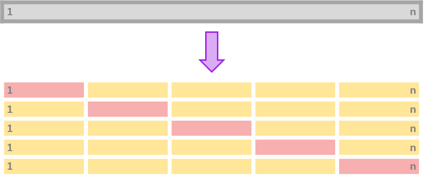ross-Validation

Procedure for k-fold cross-validation:

1. Divide your data in k-folds (usually, $K=5$ or $K=10$).

2. Use $k=1$ as the testing data and $k=2,..,K$ as the training data.

3. Calculate the accuracy measure $A_k$ on the testing data.

4. Repeat for each $k$.

5. Average $A_k$ for all $k\in K$.

Main advantage: Use the entire dataset for training AND testing.

How do we do CV in R?

library(caret)
set.seed(100)
train.control = trainControl(method = "cv", number = 10)
lm_simple = train(logins ~ succession + city, data = disney, method="lm", 
                  trControl = train.control)
lm_simple

How do we do CV in R?

library(caret) 
set.seed(100)
train.control = trainControl(method = "cv", number = 10)
lm_simple = train(logins ~ succession + city, data = disney, method="lm", 
                  trControl = train.control)
lm_simple

How do we do CV in R?

library(caret) 
set.seed(100)
train.control = trainControl(method = "cv", number = 10)
lm_simple = train(logins ~ succession + city, data = disney, method="lm", 
                  trControl = train.control)
lm_simple

How do we do CV in R?

library(caret) 
set.seed(100)
train.control = trainControl(method = "cv", number = 10)
lm_simple = train(logins ~ succession + city, data = hbo, method="lm",
                  trControl = train.control)
lm_simple

## Linear Regression 
## 
## 5000 samples
##    2 predictor
## 
## No pre-processing
## Resampling: Cross-Validated (10 fold) 
## Summary of sample sizes: 4500, 4501, 4499, 4500, 4500, 4501, ... 
## Resampling results:
## 
##   RMSE      Rsquared   MAE     
##   2.087314  0.6724741  1.639618
## 
## Tuning parameter 'intercept' was held constant at a value of TRUE

Stepwise selection

• We have seen how to choose between some given models. But what if we want to test all possible models?

• Stepwise selection: Computationally-efficient algorithm to select a model based on the data we have (subset selection).

Algorithm for forward stepwise selection:

1. Start with the null model, $M_0$ (no predictors)

2. For $k=0,...,p-1$: (a) Consider all $p-k$ models that augment $M_k$ with one additional predictor. (b) Choose the best among these $p-k$ models and call it $M_{k+1}$.

3. Select the single best model from $M_0,...,M_p$ using CV.

Backwards stepwise follows the same procedure, but starts with the full model.

How do we do stepwise selection in R?

set.seed(100)
train.control = trainControl(method = "cv", number = 10) #set up a 10-fold cv
lm.fwd = train(logins ~ . - unsubscribe, data = train.data, 
               method = "leapForward",
               tuneGrid = data.frame(nvmax = 1:5), trControl = train.control)
lm.fwd$results

##   nvmax     RMSE  Rsquared      MAE     RMSESD RsquaredSD      MAESD
## 1     1 2.269469 0.6101788 1.850376 0.04630907 0.01985045 0.04266950
## 2     2 2.087184 0.6702660 1.639885 0.04260047 0.01784601 0.04623508
## 3     3 2.087347 0.6702094 1.640405 0.04258030 0.01804773 0.04605074
## 4     4 2.088230 0.6699245 1.641402 0.04270561 0.01808685 0.04620206
## 5     5 2.088426 0.6698623 1.641528 0.04276883 0.01810569 0.04624618

• Which one would you choose out of the 5 models? Why?

How do we do stepwise selection in R?

# We can see the number of covariates that is optimal to choose:
lm.fwd$bestTune

##   nvmax
## 2     2

# And how does that model looks like:
summary(lm.fwd$finalModel)

## Subset selection object
## 5 Variables  (and intercept)
##            Forced in Forced out
## id             FALSE      FALSE
## female         FALSE      FALSE
## city           FALSE      FALSE
## age            FALSE      FALSE
## succession     FALSE      FALSE
## 1 subsets of each size up to 2
## Selection Algorithm: forward
##          id  female city age succession
## 1  ( 1 ) " " " "    " "  " " "*"       
## 2  ( 1 ) " " " "    "*"  " " "*"

# If we want the RMSE
rmse(lm.fwd, test.data)

## [1] 2.089868

Takeaway points

Next class

References

• James, G. et al. (2021). "Introduction to Statistical Learning with Applications in R". Springer. Chapter 2, 5, and 6.

• STDHA. (2018). "Stepwise Regression Essentials in R."

• STDHA. (2018). "Cross-Validation Essentials in R."