STA 235H - Classification and Regression Trees (CART)

class: center, middle, inverse, title-slide

.title[
# STA 235H - Classification and Regression Trees (CART)
]
.subtitle[
## Fall 2023
]
.author[
### McCombs School of Business, UT Austin
]

---

.small .remark-code { /*Change made here*/
  font-size: 80% !important;
}

.tiny .remark-code { /*Change made here*/
 font-size: 80% !important;
}
</style>

# Announcements

- Next week will be the **.darkorange[last class with new material]**.

- The final week of class will be for a **.darkorange[review session]**.

- Final Trivia!
  
--

- You need to choose a topic for **.darkorange[Homework 6]**

- Remember that this homework cannot be dropped.
  - All tasks have the same difficulty.
  - You will only be competing with people that choose your same dataset.

---
# Where we've been...

.pull-left[
- Talking about **.darkorange[bias vs variance]** trade-off.

- **.darkorange[Linear models, model selection and regularization]**:

- Linear regressions.
  - Stepwise selection.
  - Ridge and Lasso regression.

]

.pull-right[
.center[
![](https://media.giphy.com/media/xld5ngDPQm1piFSYUe/source.gif)
]
]

---
# ... and where we're going.

.pull-left[
.center[
![](https://media.giphy.com/media/xT5LMAsVINr1Zwsjmw/giphy.gif)
]
]

.pull-right[
- Continue on our **.darkorange[prediction]** journey:

- **.darkorange[Decision Trees]**: Classification and Regression Trees (CART)

- **.darkorange[Activity in R]**: Remember to try to complete it before the end of the class!

]
---
# Before we start... knowledge check!

- Ridge and lasso regression **.darkorange[add bias to a linear model to reduce variance]**:

- Remember that when we fit a ridge or lasso regression, we use all the predictors we have in our data!
  
--

- `$\lambda$` represents the **.darkorange[ridge/lasso penalty]**: The larger the `$\lambda$` the smaller the (sum of) coefficients, e.g. `$\sum_k\beta_k^2$` or `$\sum_k|\beta_k|$`.

- We "mute" or decrease the relation between predictors and outcome.

--

.box-7Trans[Q1: What is the main difference (in terms of the final model) between Ridge and Lasso regression?]

---
background-position: 50% 50%
class: left, bottom, inverse
.big[
Trees, trees everywhere!
]

---

.center2[
.box-5Trans[From the videos/readings, how would you explain to someone what a decision tree is?]
]

---
# Idea behind Decision Trees

- Create a **.darkorange[flow chart]** for making decisions

- *How do we classify an individual or what value do we assign to an observation?*
  
--

- ... But there are **.darkorange[many]** decisions!

--
  
  - How many variables do we use?
  
--

- How do we sort them? In what order do we place them?
  
--

- How do we split them?
  
--

- How deep do we go?

---

.center2[
.box-6Trans[Q2: What is the main disadvantage of a shallower tree (compared to a deeper tree)?]

.box-6trans[a) Higher variance 
b) Higher bias 
c) Lower variance 
d) Lower bias]
]

---
# Structure of Decision Trees

.pull-left[
.center[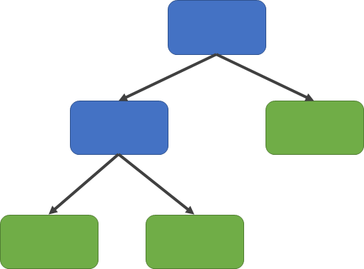
![](https://raw.githubusercontent.com/maibennett/sta235/main/exampleSite/content/Classes/Week12/1_DecisionTrees/images/tree_example.png)]
]

.pull-right[
**.darkorange[Structure:]**

- Root node
  - Internal nodes
  - Leaves
]

---
# Why do we like/not like Decision Trees?

.pull-left[
.box-4[Main advantages]
 
.box-4t[Simple interpretation]
 
.box-4t[Mirror human decision-making]
 
.box-4t[Graphic displays!]
 
.box-4t[Handle categorical variables]
]

.pull-left[
.box-6[Main disadvantages]
 
.box-6t[Overfitting]
 
.box-6t[Not very accurate/not very robust]
]

---
# Let's start with a simple example

.box-3[Remember our Hbo Max example?]

.box-3t[Predict who will cancel their subscription]

We have some **.darkorange[information:]**

- `city`: Whether the customer lives in a big city or not
- `female`: Whether the customer is female or not
- `age`: Customer's age (in years)
- `logins`: Number of logins to the platform in the past week.
- `succession`: Whether the person has watched the Succession or not.
- `unsubscribe`: Whether they canceled their subscription or not.

---
# The prediction task: Classification

- Our outcome is **.darkorange[binary]**, so this is a **.darkorange[classification task]**.

- Let's start looking at **.darkorange[two variables]**:

.box-4[City & Succession]

- Which one do you think should be at the top of the tree?

---
# How do we decide?

- **.darkorange[Recursive Binary Splitting]**:

- Divide regions of covariates in two (recursively).
  
  - This works both for continuous and categorical/binary variables
  
--

- We test out every covariate and see **.darkorange[which one reduces the error the most]** in our predictions

- In **.darkorange[regression tasks]**, we can use RMSE.
 
 - In **.darkorange[classification tasks]**, we can use accuracy/classification error rate, Gini Index, or entropy
 
--

`$$G = \sum_{k=0}^1\hat{p}_{mk}(1-\hat{p}_{mk})$$`
where `$\hat{p}_{mk}$` is the proportion of obs. in the `$m$` region for class `$k$`.
---
# How do we decide?

In our HBO Max example:

- `$k$` represents the **.darkorange[different values that the outcome]** can take (e.g. `$Unsubscribe \in \{0,1\}$`), and 
- `$m$` represents the **.darkorange[values that the predictor takes]** (e.g. `$Succession = 0$`).

E.g.:

- `$p_{mk} = p_{00}$`: The proportion of people who are subscribed (Unsubscribed = 0) and that have not watched Succession (Succession = 0)
 - `$p_{mk} = p_{01}$`: The proportion of people who are unsubscribed (Unsubscribed = 1) and that have not watched Succession (Succession = 0)
 
 
- Usually, you want the Gini index to be **.darkorange[small]**!

---

.center2[
.box-6Trans[Q3: According to the Gini Index, is it better or worse to have a high pmk (i.e. closer to 1)?]
 
 
`$$G = \sum_{k=1}^K\hat{p}_{mk}(1-\hat{p}_{mk})$$`
]

---
# Choosing predictors

- From the previous exercise, we can see that **.darkorange[using `succession` yields a lower Gini compared to `city`]** (0.428 vs. 0.482)

--
 
 
.box-2[But we have more variables]

.box-3[How do we choose?]

---
# Basic Algorithm

.box-2s[1) Start at the root node]
 
 
--
.box-4s[2) Split the parent node at covariate xi to minimize the sum of child node impurities]
 
 
--
.box-5s[3) Stop if leaves are pure or early stopping criteria is satisfied, else repeat step (1) and (2) for each new child nodes]
 
 
--
.box-6s[4) Prune your tree according to a complexity parameter (cp)]
 
 
--
.box-7s[5) Assign the average outcome (regression) or the majority (classification) in each leaf.]

.source[Adapted from "Machine Learning FAQs" (Raschka, 2021)]

---
# Grow full tree and prune it

.center[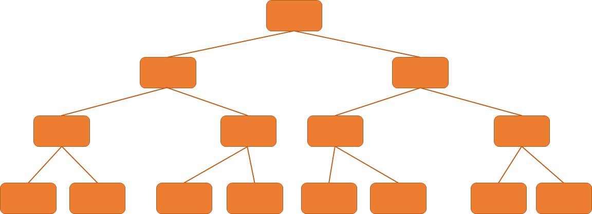
![](https://raw.githubusercontent.com/maibennett/sta235/main/exampleSite/content/Classes/Week12/1_DecisionTrees/images/full_tree.png)
]

---
# Hyper-parameter: Complexity parameter

- Measure of how much a split should **.darkorange[improve prediction]** for it to be worth it.

`$$\sum_{m=1}^{|T|} \sum_{i: i \in R_m} (y_i - \hat{y}_i)^2 + \alpha|T|$$`

- `$|T|$`: Number of terminal nodes or leaves (e.g. size of the tree)
- `$R_m$`: Predictor space of the `$m$`th leaf
- `$\alpha$`: Tuning parameter

What happens if `$\alpha=0$`?

---
# Only attempt a split if it's worth it

.center[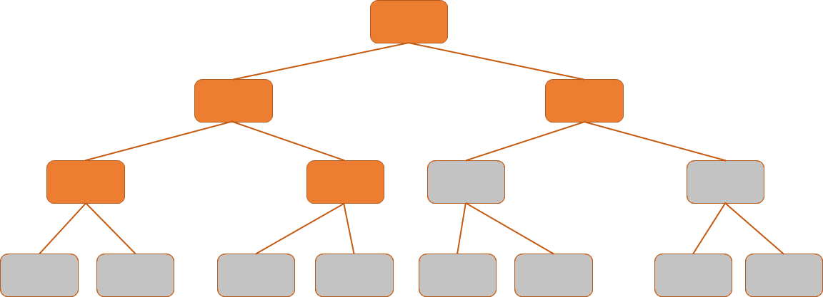
![](https://raw.githubusercontent.com/maibennett/sta235/main/exampleSite/content/Classes/Week12/1_DecisionTrees/images/not_full_tree.png)
]
---
# Let's see how to do it in R!

```r
*library(caret)

set.seed(100)

ct = train(
  factor(unsubscribe) ~ . - id, data = hbo.train, #remember your outcome needs to be a factor!
  method = "rpart", # The method is called rpart
  trControl = trainControl("cv", number = 10),
  tuneLength = 15
)
```
---
# Let's see how to do it in R!

```r
library(caret)

set.seed(100)

ct = train(
  factor(unsubscribe) ~ . - id, data = hbo.train, #remember your outcome needs to be a factor!
* method = "rpart",
  trControl = trainControl("cv", number = 10),
  tuneLength = 15
)
```

---
# Let's see how to do it in R!

```r
library(caret)

set.seed(100)

ct = train(
  factor(unsubscribe) ~ . - id, data = hbo.train, #remember your outcome needs to be a factor!
  method = "rpart",
  trControl = trainControl("cv", number = 10),
* tuneLength = 15
)
```

- `tuneLength` is useful when you don't want to pass a specific grid (usually it might not be enough though!)

---
# We could also provide a grid of complexity parameters

```r
library(rpart)

set.seed(100)

ct = train(
  factor(unsubscribe) ~ . - id, data = hbo.train,
  method = "rpart",
  trControl = trainControl("cv", number = 10),
* tuneGrid = expand.grid(cp = seq(0,1, by = 0.01)),
  control = rpart.control(minsplit = 20)
)
```
.small[
- `cp`: Complexity parameter

- Split must decrease the overall lack of fit by a factor of `cp`, or is not attempted.
  
  - Parameter for **.darkorange[pruning the tree]**.
  
  - Higher `cp`, smaller the tree!

- `minsplit`: Min. number of obs in a node to attempt a split.]

---
# This works similarly to the penalty term in regularization...
.small[

```r
plot(ct)
```

```r
ct$bestTune
```

```
##     cp
## 4 0.03
```
]

---
# ... And we can also plot the tree!

.small[

```r
library(rattle)

fancyRpartPlot(ct$finalModel, caption = "Classification tree for Unsubscribe")
```

<img src="f2023_sta235h_12_DecisionTrees_files/figure-html/full_tree-1.svg" style="display: block; margin: auto;" />
]

---
 
.box-4Trans[What do you think the percentages in the leaves represent?]

<img src="f2023_sta235h_12_DecisionTrees_files/figure-html/full_tree2-1.svg" style="display: block; margin: auto;" />
 
---
background-position: 50% 50%
class: left, bottom, inverse
.big[
Regression Trees
]
---
# Regression Trees

- Outcome is **.darkorange[continuous]**

- Very similar to what we have seen with **.darkorange[classification trees]**:

- Predicted outcome is the **.darkorange[mean outcome for the leaf/region]**.

---
# In R is basically the same

.pull-left[

```r
set.seed(100)

rt = train(
  logins ~. - unsubscribe - id, data = hbo.train, 
  method = "rpart",
  trControl = trainControl("cv", number = 10),
  tuneLength = 20
  )

plot(rt)
```
]

.pull-right[
<img src="f2023_sta235h_12_DecisionTrees_files/figure-html/plot_cv-1.svg" style="display: block; margin: auto;" />
]

---
# Providing a specific grid for cp

.pull-left[

```r
set.seed(100)

*tuneGrid = expand.grid(cp = seq(0, 0.1, by = 0.005))

rt = train(
  logins ~. - unsubscribe - id, data = hbo.train, 
  method = "rpart",
  trControl = trainControl("cv", number = 10),
* tuneGrid = tuneGrid
  )

plot(rt)
```
]

.pull-right[
<img src="f2023_sta235h_12_DecisionTrees_files/figure-html/plot_cv2-1.svg" style="display: block; margin: auto;" />
]

---
# Plot the tree

.pull-left[

```r
fancyRpartPlot(rt$finalModel, caption="Regression Tree for Login")
```

<img src="f2023_sta235h_12_DecisionTrees_files/figure-html/plot_tree_reg-1.svg" style="display: block; margin: auto;" />
]

.pull-right[

```r
rt$finalModel
```

```
## n= 5000 
## 
## node), split, n, deviance, yval
## * denotes terminal node
## 
## 1) root 5000 66387.3700 4.806800 
## 2) succession>=0.5 3535 24633.5000 2.973409 
## 4) city< 0.5 500 517.1580 0.322000 *
## 5) city>=0.5 3035 20022.2800 3.410214 *
## 3) succession< 0.5 1465 1200.0180 9.230717 
## 6) city< 0.5 212 132.2028 8.061321 *
## 7) city>=0.5 1253 728.8571 9.428571 *
```
]

---
.box-6Trans[Q4: What would the predicted value be for a customer who hasn't watched Succession and lives in a city?]

.pull-left[

```r
fancyRpartPlot(rt$finalModel, caption="Regression Tree for Login")
```

<img src="f2023_sta235h_12_DecisionTrees_files/figure-html/plot_tree_reg2-1.svg" style="display: block; margin: auto;" />
]

.pull-right[

```r
rt$finalModel
```

---
# Main takeaways of decision trees

.pull-left[
.center[
![](https://media.giphy.com/media/1xOyKwXRD0a96CcCfT/giphy.gif)
]
]

.pull-right[
**.darkorange[Main advantages:]**

- Easy to interpret and explain (you can plot them!)
  
- Mirrors human decision-making.
  
- Can handle qualitative predictors (without need for dummies).
  
**.darkorange[Main disadvantages:]**

- Accuracy not as high as other methods
  
  - Very sensitive to training data (e.g. overfitting)
]

---
# Next class

.pull-left[
Use of decision trees as building blocks for **.darkorange[more powerful prediction methods!]**

- Bagging
  
- Random Forests
  
- Boosting]

.pull-right[
.center[
![](https://media.giphy.com/media/cRH5deQTgTMR2/giphy.gif)
]
]

---
# References

- James, G. et al. (2021). "Introduction to Statistical Learning with Applications in R". *Springer. Chapter 8*

- Starmer, J.. (2018). "Decision Trees". *Video materials from StatQuest (YouTube)*.

- STDHA. (2018). ["CART Model: Decision Tree Essentials"](http://www.sthda.com/english/articles/35-statistical-machine-learning-essentials/141-cart-model-decision-tree-essentials)